


Series Intro#
In this series, I will share my experiences in contributing to open source software. I have really enjoyed contributing back to libraries that have been useful in my career, and want to encourage and inspire others to jump in and do the same!
Background#
One of the foundational activities when trying to assess data quality at scale is data profiling. Put simply, it’s analyzing high-level exploratory metrics like:
- Row Counts
- Numerical column statistics (mean, median, distributions)
- Categorical column information (distinct values, distinct counts)
- Fill rates of columns (how many are null?)
Last year, my team was asked to perform a large-scale data quality initiative, so we had a need for an efficient process that could deliver exploratory insights in a repeatable fashion.
We needed a process that supported tables with tens of millions of records, most of which are delta lake tables in our data lake, and we landed on a tool called fg-data-profiling.
The tagline itself describes exactly why we like it:
1 Line of code data quality profiling & exploratory data analysis for Pandas and Spark DataFrames.
Using fg-data-profiling#
With just a couple lines of code, you get a nice fancy HTML export that you can explore and share:
import numpy as np
import pandas as pd
from data_profiling import ProfileReport

df = pd.DataFrame(np.random.rand(100, 5), columns=["a", "b", "c", "d", "e"])

profile = ProfileReport(df, title="YData Profiling Report")

profile.to_file("your_report.html")
Which would produce an output that looks like this:
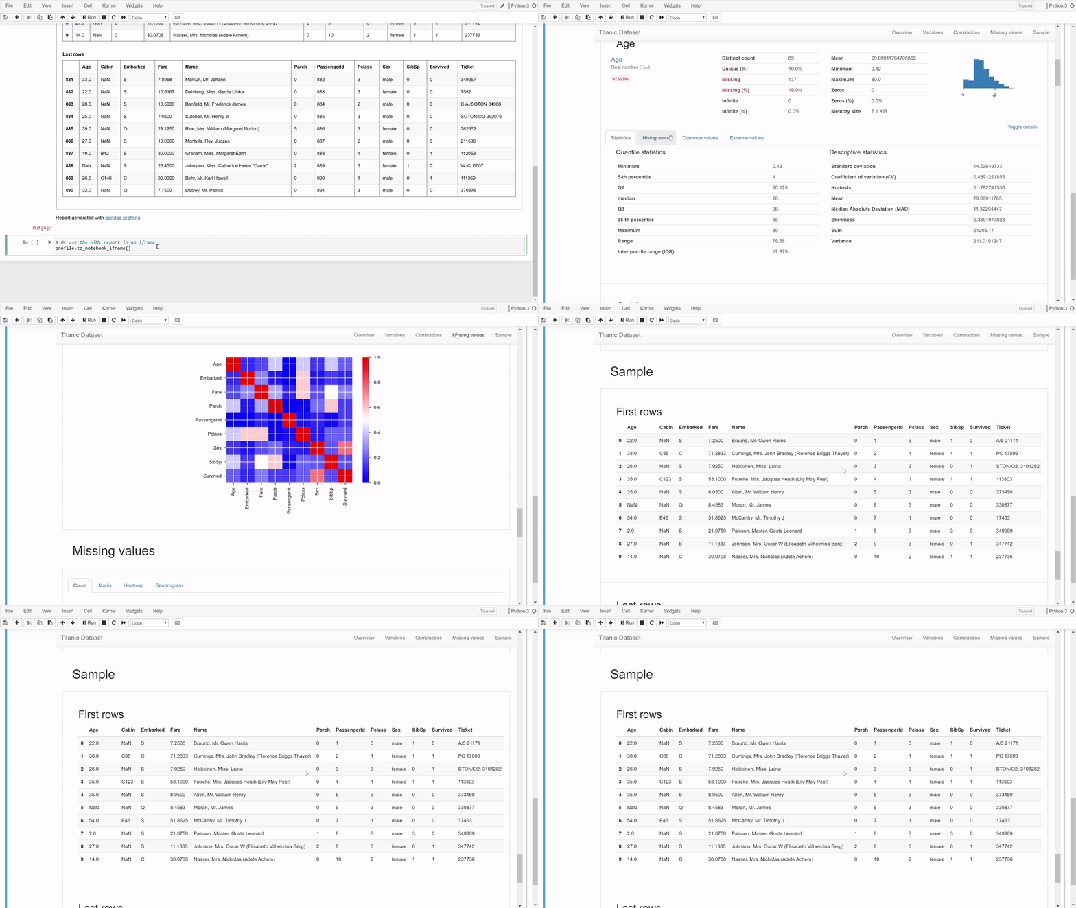
This image is from their documentation at https://docs.profiling.ydata.ai/.
What is ydata-profiling? They just re-branded to fg-data-profiling.
A Case for Spark#
That example uses pandas to run a profile on that DataFrame, which is great when data is small and fits in memory easily.
At the time, my team was testing this all out in our Azure Synapse implementation.
The profiles were taking ~20+ minutes initially because this code was running pandas directly on the driver node, and not taking advantage of the entire Spark cluster.
For the volume of data my team was profiling, we needed to leverage Spark so that all the heavy lifting would happen in our Spark Cluster.
Good thing fg-data-profiling supports Spark DataFrames!
The same profiles that were taking 20+ minutes were now running in ~2 minutes - a 10x speedup!
Time to celebrate?! Well…
The Problem#
Running the data profiling in Spark was fast, however, when we compared those outputs to our slower examples in pandas, we noticed that they produced completely different results. (In data, it’s always good to be skeptical and constantly verify EVERYTHING). This didn’t sit well with me, so I decided to dive into the library’s implementation to see what could possibly be different.
Luckily, this library is written in pure python, so it was incredibly easy to reason through how the profiling works under the hood. Here is how I approached discovering the differences:
Test Driven Development#
I find Test Driven Development one of the best ways to not only build new software, but also explore bugs and assumptions about behavior. In this case, the assumption is:
Given the same dataset, the data profile report should be the same for pandas and Spark
Sounds like a reasonable assumption, so I built a toy dataset to test this theory:
from typing import List, Optional, Tuple

from pyspark.sql import types as T

RowType = Tuple[
    Optional[str],
    Optional[float],
    Optional[int],
    Optional[bool],
    Optional[float],
    Optional[str],
]


def create_test_df(spark: SparkSession) -> DataFrame:
    schema = T.StructType(
        [
            T.StructField("category", T.StringType(), True),
            T.StructField("double", T.DoubleType(), True),
            T.StructField("int", T.IntegerType(), True),
            T.StructField("boolean", T.BooleanType(), True),
            T.StructField("null_double", T.DoubleType(), True),
            T.StructField("null_string", T.StringType(), True),
        ]
    )

    data: List[RowType] = [
        (f"test_{num + 1}", float(num), int(num), True, None, None)
        for num in range(205)
    ]

    # Adding dupes
    data.extend([("test_1", float(1), int(1), False, None, None) for _ in range(205)])

    # Adding nulls
    data.extend([(None, None, None, None, None, None) for _ in range(100)])

    return spark.createDataFrame(data, schema=schema)
There are some key features about this data that we should see in the profile:
- There’s a field for every type that was having issues
- We duplicate a bunch of the numeric values to ensure the distribution is skewed
- We duplicate a categorical field to also show a skewed distribution
- We add a sizable amount of nulls, including columns that are always null
Now we can run the profile, once for pandas, then for Spark and compare the outputs.
from data_profiling import ProfileReport

# ... assuming we have a spark session as the `spark` variable

spark_df = create_test_df(spark)
pandas_df = spark_df.toPandas()

pandas_profile = ProfileReport(pandas_df, title="Pandas Profiling Report")
spark_profile = ProfileReport(spark_df, title="Spark Profiling Report")

pandas_profile.to_file("pandas_example.html")
spark_profile.to_file("spark_example.html")
Initial State - pandas#
Here is what that initial profile looks like when run with a pandas dataframe:
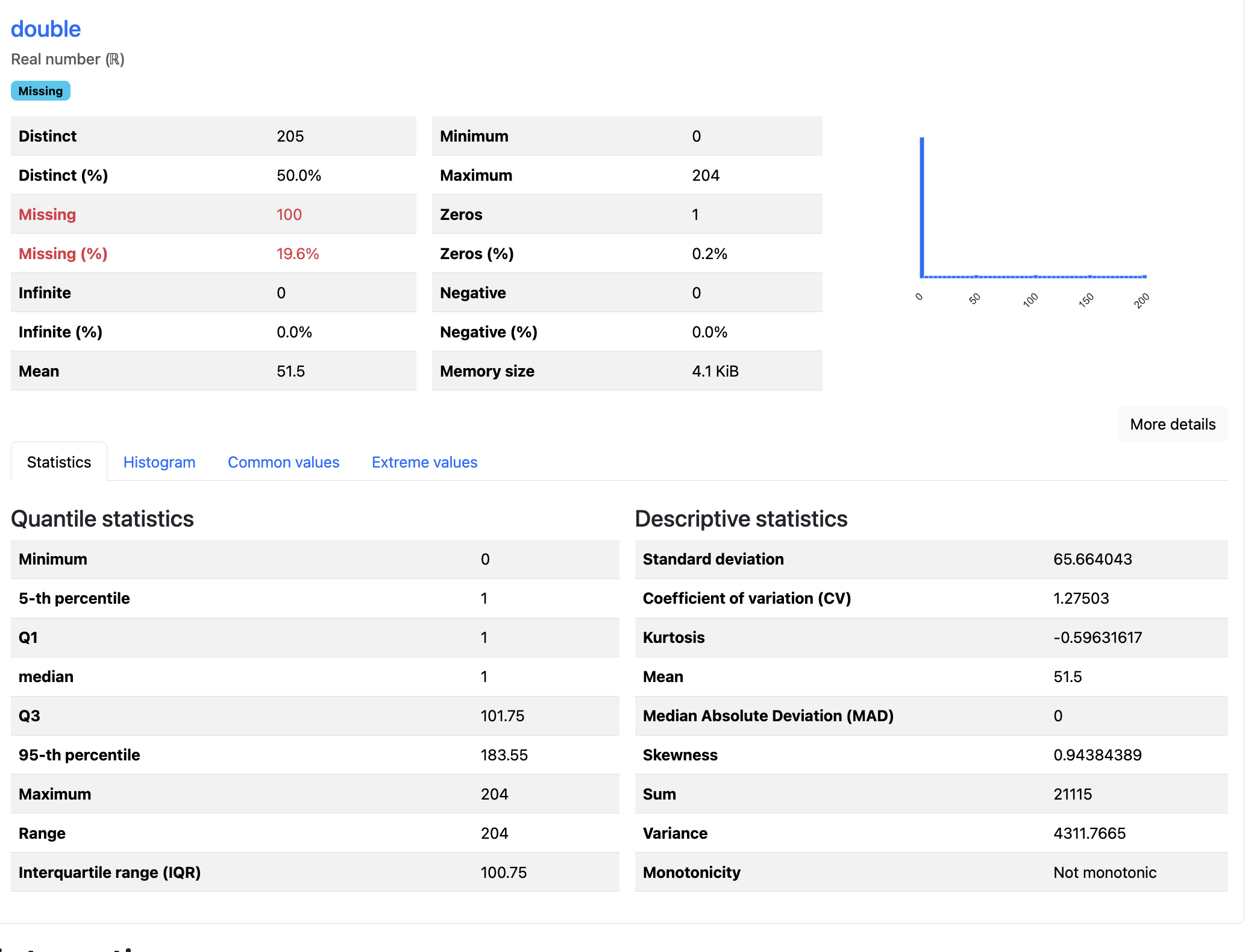
pandas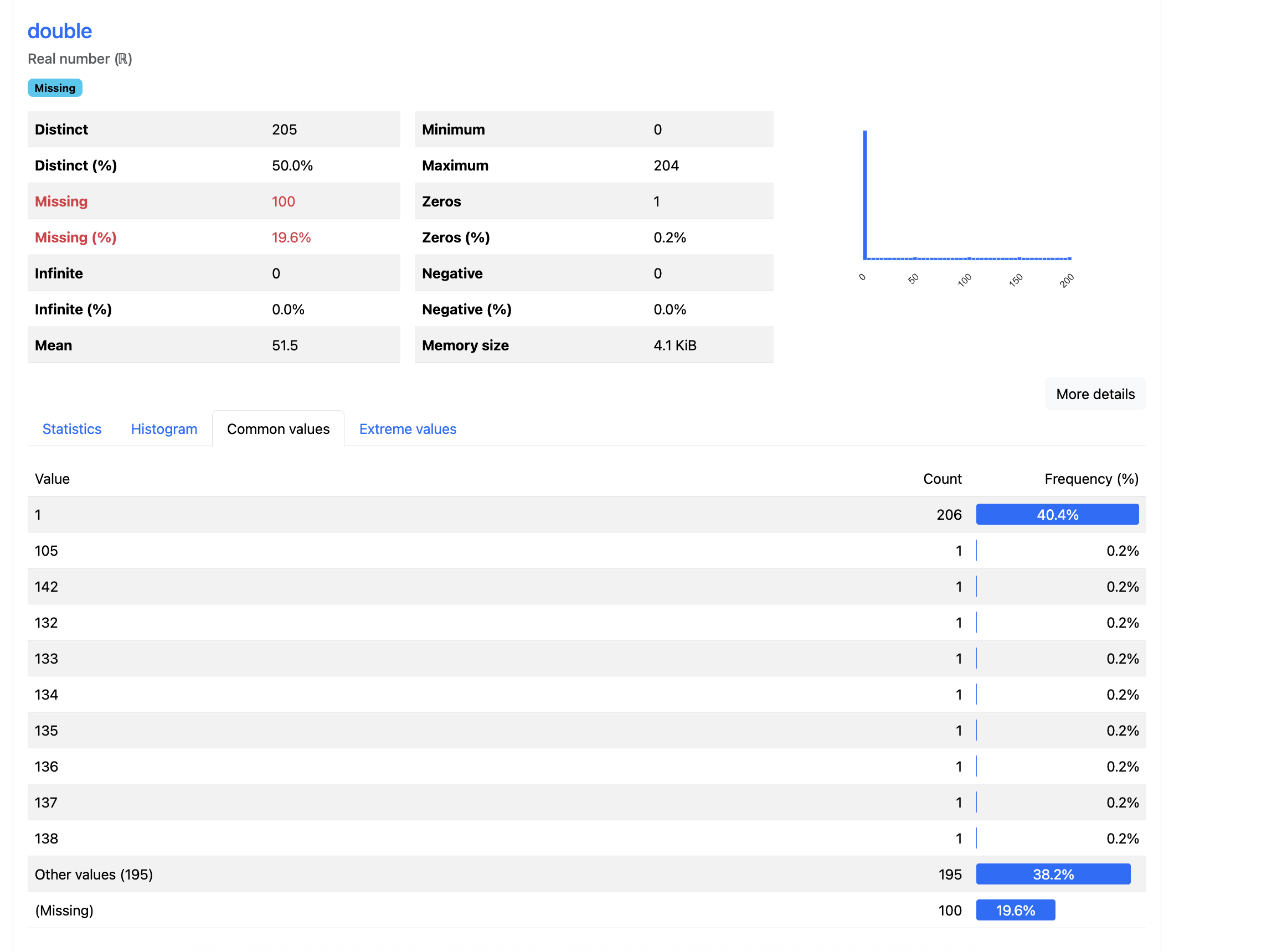
pandas (common values)Initial State - Spark#
But here is what that same dataset looked like when profiled in Spark:
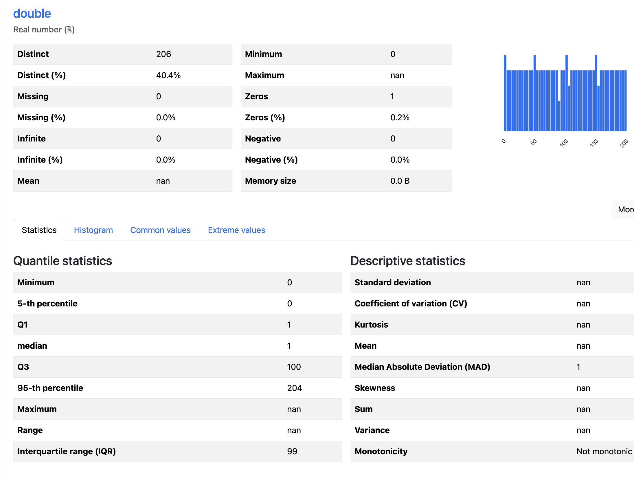
Spark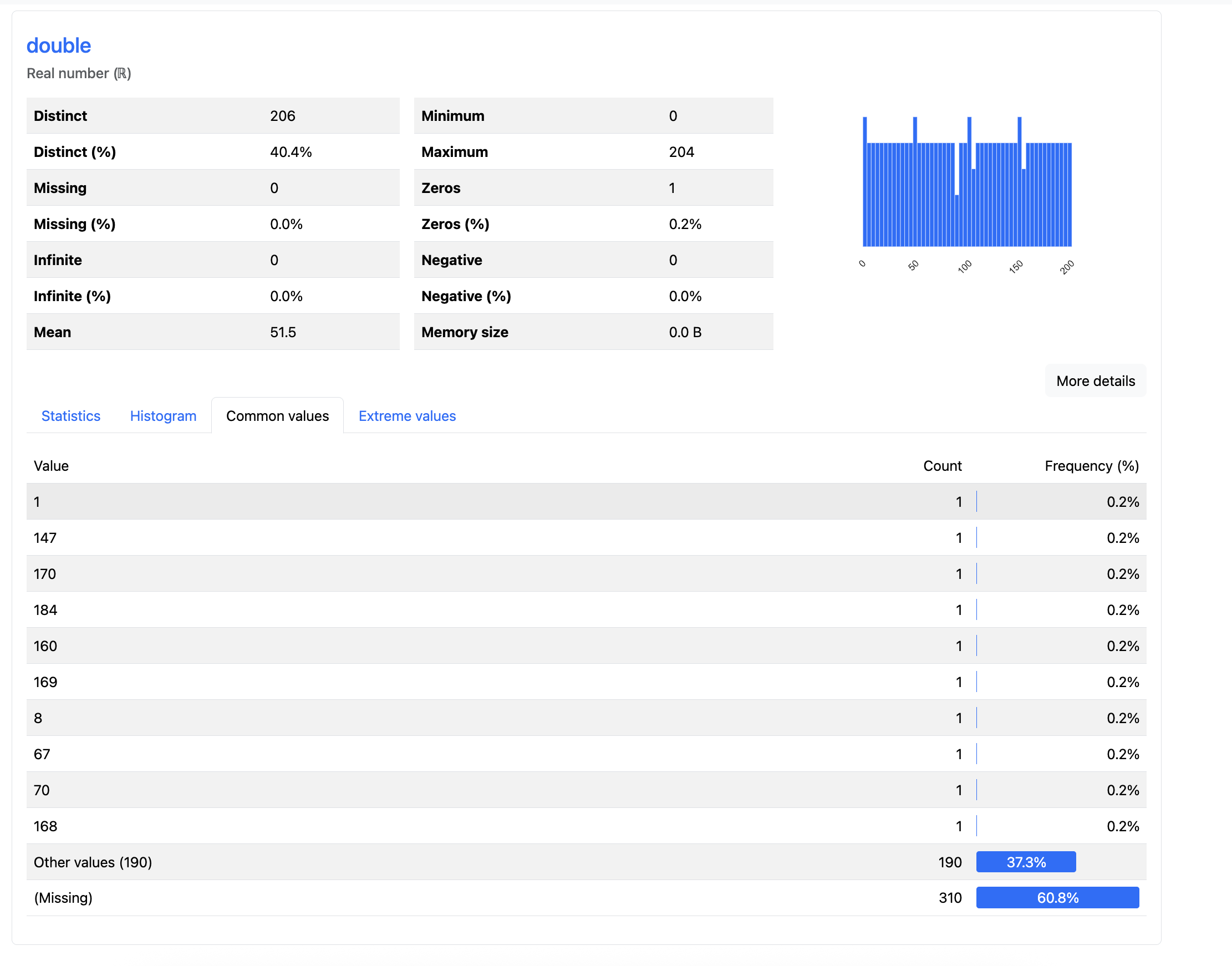
Spark (common values)Clearly there are some glaring differences in the output.
- Spark shows a flat distribution of values, when the actual data shows that the value of 1 is duplicated far more
- The missing count in Spark shows
310, but we know there are only100missing values - Most of the descriptive stats in Spark are
nanor far off from pandas
Now that we have a small, controlled dataset as our baseline, and we have these observed failures, we can now dig into the source code and figure out what needs to be fixed.
The Solution#
There were a lot of changes that went into the PR I put up to resolve each of these issues. Let’s walk through each of the main problems and their solutions based on the key changes that were made in that PR.
Fixing Flat Distribution#
To fix the flat distribution of distinct values, here are the relevant code changes:
diff --git a/src/ydata_profiling/model/spark/describe_counts_spark.py b/src/ydata_profiling/model/spark/describe_counts_spark.py
index d7a091e7f..f02d1043c 100644
--- a/src/ydata_profiling/model/spark/describe_counts_spark.py
+++ b/src/ydata_profiling/model/spark/describe_counts_spark.py
@@ -6,6 +6,7 @@
5 import pandas as pd
6 from pyspark.sql import DataFrame
7 from pyspark.sql import functions as F
8+from pyspark.sql import types as T
9
10 from ydata_profiling.config import Settings
11 from ydata_profiling.model.summary_algorithms import describe_counts
@@ -25,6 +26,11 @@
25 def describe_counts_spark(
26 Returns:
27 Updated settings, input series, and summary dictionary.
28 """
29+ # Cast Decimal Type s
30+ if isinstance(series.schema.fields[0].dataType, T.DecimalType):
31+ series = series.select(
32+ F.col(series.columns[0]).cast(T.DoubleType()).alias(series.columns[0])
33+ )
34
35 # Count occurrences of each value
36 value_counts = series.groupBy(series.columns[0]).count()
@@ -36,9 +42,23 @@
41 def describe_counts_spark(
42 value_counts_index_sorted = value_counts.orderBy(F.asc(series.columns[0]))
43
44 # Count missing values
- n_missing = (
- value_counts.filter(F.col(series.columns[0]).isNull()).select("count").first()
- )
45+ if series.dtypes[0][1] in ("int", "float", "bigint", "double"):
46+ n_missing = (
47+ # Need to add the isnan() check because Pandas isnull check will count NaN as null, but Spark does not
48+ value_counts.filter(
49+ F.col(series.columns[0]).isNull() | F.isnan(F.col(series.columns[0]))
50+ )
51+ .select("count")
52+ .first()
53+ )
54+ else:
55+ n_missing = (
56+ # Need to add the isnan() check because Pandas isnull check will count NaN as null, but Spark does not
57+ value_counts.filter(F.col(series.columns[0]).isNull())
58+ .select("count")
59+ .first()
60+ )
61+
62 n_missing = n_missing["count"] if n_missing else 0
63
64 # Convert top 200 values to Pandas for frequency table display
@@ -60,17 +80,15 @@
79 def describe_counts_spark(
80 value_counts.filter(F.col(column).isNotNull()) # Exclude NaNs
81 .filter(~F.isnan(F.col(column))) # Remove implicit NaNs (if numeric column)
82 .groupBy(column) # Group by unique values
- .count() # Count occurrences
83+ .agg(F.sum("count").alias("count")) # Sum of count
84 .orderBy(F.desc("count")) # Sort in descending order
- .limit(200) # Limit for performance
85 )
86 else:
87 value_counts_no_nan = (
88 value_counts.filter(F.col(column).isNotNull()) # Exclude NULLs
89 .groupBy(column) # Group by unique timestamp values
- .count() # Count occurrences
90+ .agg(F.sum("count").alias("count")) # Sum of count
91 .orderBy(F.desc("count")) # Sort by most frequent timestamps
- .limit(200) # Limit for performance
92 )
93
94 # Convert to Pandas Series, forcing proper structure
The problem here in the original code the produces the profile for a single column. It was running a count on an already aggregated dataframe:
value_counts = series.groupBy(series.columns[0]).count()

...

if series.dtypes[0][1] in ("int", "float", "bigint", "double"):
        value_counts_no_nan = (
            value_counts.filter(F.col(column).isNotNull())  # Exclude NaNs
            .filter(~F.isnan(F.col(column)))  # Remove implicit NaNs (if numeric column)
            .groupBy(column)  # Group by unique values
            .count()  # Count occurrences
            .orderBy(F.desc("count"))  # Sort in descending order
            .limit(200)  # Limit for performance
        )
else:
    value_counts_no_nan = (
        value_counts.filter(F.col(column).isNotNull())  # Exclude NULLs
        .groupBy(column)  # Group by unique timestamp values
        .count()  # Count occurrences
        .orderBy(F.desc("count"))  # Sort by most frequent timestamps
        .limit(200)  # Limit for performance
    )
With our test dataset that we created, we should have numbers 1 - 205, with 1 being duplicated many times, so the value_counts dataframe would be a table like this:
| decimal | count |
|---|---|
| 1 | 206 |
| 2 | 1 |
| 3 | 1 |
| … | … |
| 205 | 1 |
But the original code was running a .count() on that aggregated dataset, so the resulting table ended up just counting the rows like this:
| decimal | count |
|---|---|
| 1 | 1 |
| 2 | 1 |
| 3 | 1 |
| … | … |
| 205 | 1 |
That leaves every value at a flat count of 1 for every unique variable and not the actual distribution like we expect. The solution is to switch to a sum of the count column:
value_counts = series.groupBy(series.columns[0]).count()

...

if series.dtypes[0][1] in ("int", "float", "bigint", "double"):
        value_counts_no_nan = (
            value_counts.filter(F.col(column).isNotNull())  # Exclude NaNs
            .filter(~F.isnan(F.col(column)))  # Remove implicit NaNs (if numeric column)
            .groupBy(column)  # Group by unique values
            .agg(F.sum("count").alias("count"))  # Sum of count
            .orderBy(F.desc("count"))  # Sort in descending order
        )
else:
    value_counts_no_nan = (
        value_counts.filter(F.col(column).isNotNull())  # Exclude NULLs
        .groupBy(column)  # Group by unique timestamp values
        .agg(F.sum("count").alias("count"))  # Sum of count
        .orderBy(F.desc("count"))  # Sort by most frequent timestamps
    )
Now the distribution is fixed!
Fixing Missing Count#
In that same fix above, we resolved the proper “Missing” counts by removing the limit(200) line.
That makes sure all records were returned, because it’s basing everything off of the total row count.
When it was limiting to the top 200 records, then any row that wasn’t in the top 200 was considered “missing” even though it wasn’t null.
Another nuance here is that we needed to make sure that NaN values were counted as “Missing” as well, because Spark does NOT count those as Null:
if series.dtypes[0][1] in ("int", "float", "bigint", "double"):
        n_missing = (
            # Need to add the isnan() check because Pandas isnull check will count NaN as null, but Spark does not
            value_counts.filter(
                F.col(series.columns[0]).isNull() | F.isnan(F.col(series.columns[0]))
            )
            .select("count")
            .first()
        )
else:
    n_missing = (
        # Need to add the isnan() check because Pandas isnull check will count NaN as null, but Spark does not
        value_counts.filter(F.col(series.columns[0]).isNull())
        .select("count")
        .first()
    )
Now the output of the actual count of unique values is fixed! Let’s move onto the numerical summary issue.
Fixing Numerical Summary#
Here are the specific code changes that resolve the other numerical summary issues:
diff --git a/src/ydata_profiling/model/spark/describe_numeric_spark.py b/src/ydata_profiling/model/spark/describe_numeric_spark.py
index 5e30c7539..8c299577e 100644
--- a/src/ydata_profiling/model/spark/describe_numeric_spark.py
+++ b/src/ydata_profiling/model/spark/describe_numeric_spark.py
@@ -11,6 +11,14 @@
10 def numeric_stats_spark(df: DataFrame, summary: dict) -> dict:
11 column = df.columns[0]
12
13+ # Removing null types from numeric summary stats to match Pandas defaults which skip na's (skipna=False)
14+ finite_filter = (
15+ F.col(column).isNotNull()
16+ & ~F.isnan(F.col(column))
17+ & ~F.col(column).isin([np.inf, -np.inf])
18+ )
19+ non_null_df = df.filter(finite_filter)
20+
21 expr = [
22 F.mean(F.col(column)).alias("mean"),
23 F.stddev(F.col(column)).alias("std"),
@@ -21,7 +29,7 @@
28 def numeric_stats_spark(df: DataFrame, summary: dict) -> dict:
29 F.skewness(F.col(column)).alias("skewness"),
30 F.sum(F.col(column)).alias("sum"),
31 ]
- return df.agg(*expr).first().asDict()
32+ return non_null_df.agg(*expr).first().asDict()
33
34
35 def describe_numeric_1d_spark(
@@ -81,30 +89,42 @@
88 def describe_numeric_1d_spark(
89 quantiles = config.vars.num.quantiles
90 quantile_threshold = 0.05
91
- summary.update(
- {
- f"{percentile:.0%}": value
- for percentile, value in zip(
- quantiles,
- df.stat.approxQuantile(
- f"{df.columns[0]}",
92+ if summary.get("n") == summary.get("n_missing"):
93+ # This means the entire column is null/nan, so summary values need to be hard-coded:
94+ summary.update({f"{percentile:.0%}": np.nan for percentile in quantiles})
95+
96+ summary["mad"] = np.nan
97+ summary["iqr"] = np.nan
98+
99+ else:
100+ summary.update(
101+ {
102+ f"{percentile:.0%}": value
103+ for percentile, value in zip(
104 quantiles,
- quantile_threshold,
- ),
- )
- }
- )
105+ df.stat.approxQuantile(
106+ f"{df.columns[0]}",
107+ quantiles,
108+ quantile_threshold,
109+ ),
110+ )
111+ }
112+ )
113
- median = summary["50%"]
114+ median = summary.get("50%")
115
- summary["mad"] = df.select(
- (F.abs(F.col(f"{df.columns[0]}").cast("int") - median)).alias("abs_dev")
- ).stat.approxQuantile("abs_dev", [0.5], quantile_threshold)[0]
116+ summary["mad"] = df.select(
117+ (F.abs(F.col(f"{df.columns[0]}").cast("int") - median)).alias("abs_dev")
118+ ).stat.approxQuantile("abs_dev", [0.5], quantile_threshold)[0]
119+
120+ summary["iqr"] = summary["75%"] - summary["25%"]
121
122 # FIXME: move to fmt
123 summary["p_negative"] = summary["n_negative"] / summary["n"]
- summary["range"] = summary["max"] - summary["min"]
- summary["iqr"] = summary["75%"] - summary["25%"]
124+ if summary["min"] is None or summary["max"] is None:
125+ summary["range"] = np.nan
126+ else:
127+ summary["range"] = summary["max"] - summary["min"]
128 summary["cv"] = summary["std"] / summary["mean"] if summary["mean"] else np.nan
129 summary["p_zeros"] = summary["n_zeros"] / summary["n"]
130 summary["p_infinite"] = summary["n_infinite"] / summary["n"]
The root cause of the mismatching summary statistics is due to a difference in how pandas handles null values vs. how Spark handles that scenario.
As an example, take the documentation for the mean function in pandas.
The key observation here is:
The
skipnaargument defaults toTrue.
This means that for a column that has null values, the summary statistic to be computed filters out any null values.
In pandas, NaN values are considered null, but in Spark, NaN is considered not null and will simply return a NaN for the aggregate summary statistic.
Therefore, to match pandas’ output, our Spark solution had to filter out exactly what pandas would filter out, so things like NaN (not a number), null values, and any values representing infinity.
The other edge case we handle with our test dataset is where columns can be completely null.
These were breaking in the reports, so we forced a default NaN value when we aren’t able to actually compute the statistic.
Other Misc Fixes#
The rest of the changes in the PR handle a couple edge cases that our test data produced:
- Fixes reporting cases when a column was entirely null (certain reports would simply break or not render, so we render a placeholder instead)
- Enables the
DecimalTypein numerical stats, because we can cast that to a float and perform the same mathematical operations easily.
Fixed State - Spark vs. Pandas#
With all of these fixes, Spark’s output is now correctly matching the original pandas output:
pandas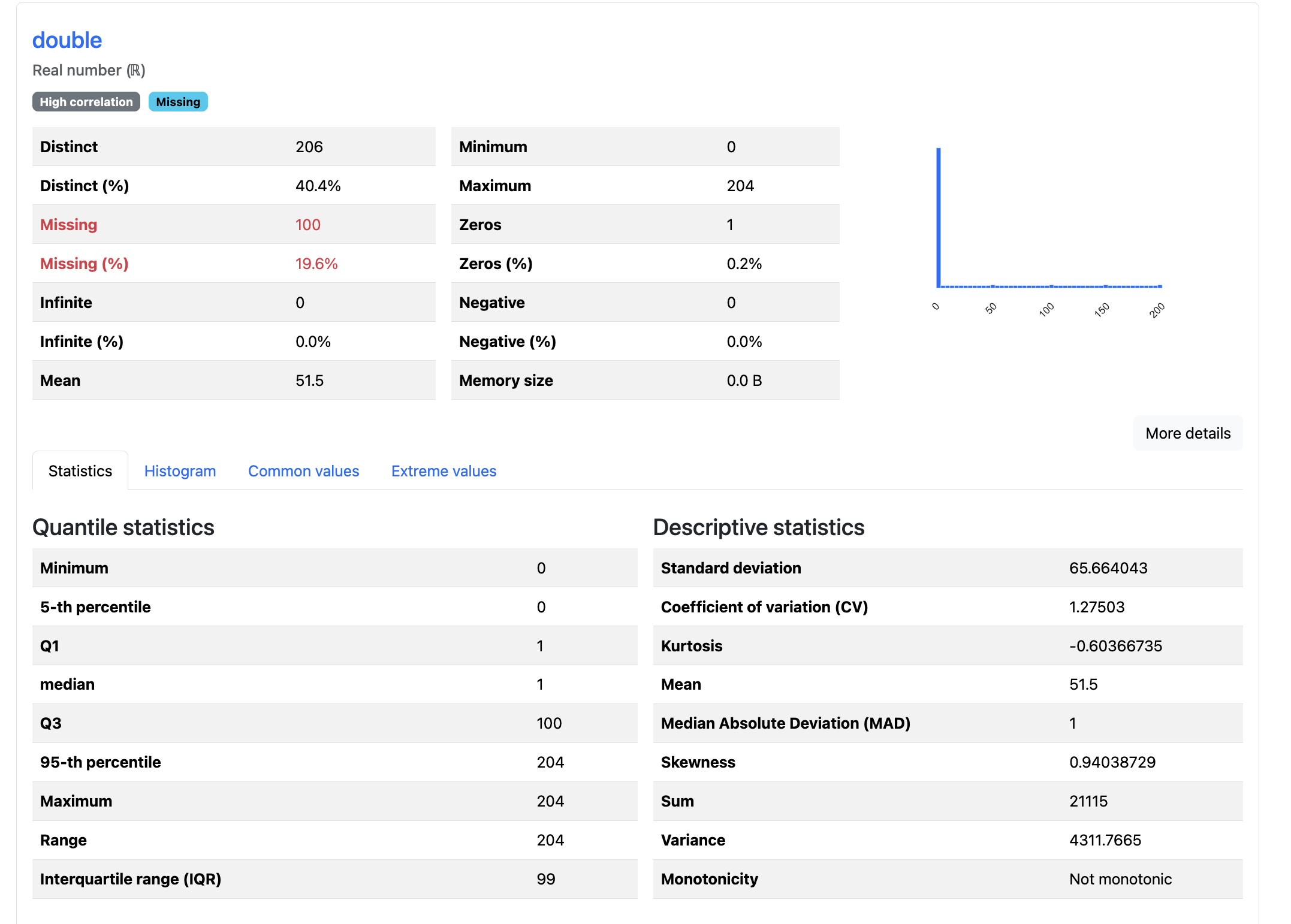
Sparkpandas (common values)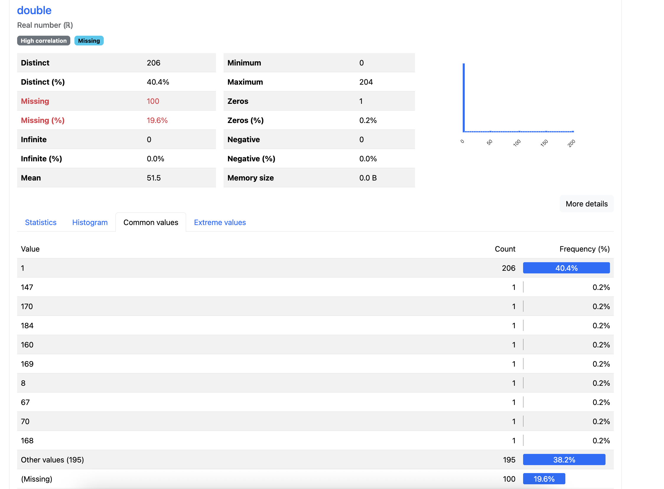
Spark (common values)Conclusion#
Once we had these changes implemented and merged, our team was able to fully leverage the fg-data-profiling tool for our data quality audit. This vastly sped up our iteration time as we could take full advantage of the Spark cluster to get the answers we needed.
When using pandas on its own, the ~10+ minutes was reading the entire source tables into memory on the driver before doing any aggregation.
Using Spark, we allowed the query engine to do most of that hard aggregation work without the need to bring the entire table into the.
At the end of the day with these fixes, our profiles still had that ~10x speedup!
Personally, this is what I consider to be my first impactful contribution to an open-source project. When I was fixing this for my team, I realized I could give back to the community by simply sharing what I found. It was incredibly rewarding to see 4 different issues resolved based on this one PR, and then to see a release cut so quickly after getting this merged!
The team who maintains fg-data-profiling was so responsive and kind in their feedback, which inspired me to seek out more opportunities to contribute to open-source projects.
Looking forward to sharing more of my adventures in open source in this series!